We have come to the final post! We have reached the end! In this post, I will comment on my final model. Let’s quickly be reminded of this model:
The R-Squared is 98% which is great. My model predicts 98% of variation in air time. That is a very high amount of variation to explain. Now let’s look at accuracy and stability.
Not all of the code fit!
First let’s look for stability. The NA does not help here and thus cannot determine if the model is stable, because there is nothing to compare it so. Next, for accuracy. The errors of these graphs seem very similar to me, so I can conclude they are accurate. Additionally, my predictions are off by 4, which talking about flights and the amount of flights happening a day, to me does not seem like a huge number. I would say this is accurate too.
In conclusion, I have learned a lot about data analytics and succeeded in it a lot more than I thought I would! My data and impact post stated I would predict flight cancellations, however I discovered some bumps in the road with that and switched my predicting variable. I did not meet my goals of what I originally set out to do. But my personal goal of learning new skills and new knowledge of this topic definitely was met! I do not believe I have the best model, but I don’t believe it is the worst. I would recommend my firm leave my model as is, use it as a predictor if needed, but invest money in a different model. I think my model is decently effective but I think there is always room for improvement. I am proud of how far I have come as a business analytics student and I thank you all for following along on this journey!
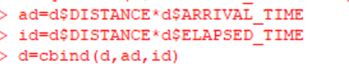
This post I will be adding interactions to my model. This is basically adding in a combination of two variables. My six variables are distance, elapsed time, scheduled departure, time and arrival along with departure delay. I can use only my significant variables in these interactions, but I also can now use insignificant variables. Now that I have created interactions, I will divide my data and create a new model with these interactions.
I have added two interactions to my data set. The interactions and code to build these interactions are shown below. This step is occurring before I divide my data, however I am using data with the outliers removed.
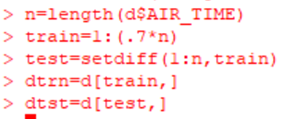
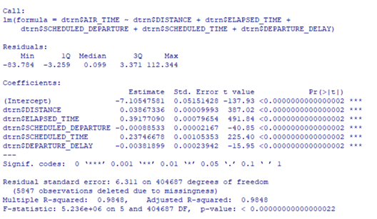
I will now divide my data and build a new model with my training set and the interactions. My output is below.
The original R-Squared was 98.36% and the new R-Squared is 98.37%. This means, the combinations of distance and arrival time, along with air time and elapsed time contribute .01% to the R-Squared. I count both of them into this because both interactions are significant. I can also include all of my predictors in my new equations because they are all significant. They do add a very small amount to my data, and they also do not hurt my model, so I will keep them.
My new model equation is:
air time=-7.08+0.04*distance+0.4*elapsedtime-0.002*scheduledarrival+0.001*scheduleddeparture+0.25*scheduledtime-0.004*departuredelay-0.000001*distance*arrivaltime-0.00002*distance*elapsedtime
My interactions tell me distance and arrival time have a positive relationship, and distance and elapsed time have a negative relationship. When distance is increased, the air time and arrival time is longer/later. Meaning, the air time is longer and thus arrival time of a flight is later, when the distance increases. Additionally, when distance is decreased, air time decreases however elapsed time increases, as it pertains to the time door to door. And we take in to account the time after and before the plane is at and gets to the the gate, whereas air time does not consider that.
Thanks for following along with me in this process! We are one post away from the end:)
Today we are going to talk about outliers, or an instance that happens out of the ordinary data, it does not follow what seems to be the “norm” of the other data. They can be bad because the are such extremes that can skew our data. I will be testing for these outliers, and if there are some, removing them from my data.
My first step is to graph air time with all of my significant predictors. By graphing, I will be able to pick out outliers if present.
Some of the models seem fine and do not have many extremes, while a few others such as scheduled arrival, departure and departure delay have a few weird parts to them. For example, there seems to be a weird island of data in the scheduled arrival along with scheduled departure, that has an air time greater than 300. Similarly, departure delay has a lot of scattered data greater than 500. This is another outlier. Now let’s check to confirm if they are outliers. We will see how many times this data occurs using the code below.
The output tells me the amount of data over 300 and 500. As shown in the graphs, this data over this amount seems to be clustered around 500 in scheduled arrival and 2000 in scheduled departure. If these values were not outliers, they would not be huddled around these values. Instead, they would be at 300 and 500, but spread out across the values of scheduled arrival and departure. These clusters are not good for the data because it can skew it. They are extremes that do not follow the rest of the data. Thus, conclusions we make may be off if we keep the outliers in our data. The next step is to remove the outliers, to help make our model more precise.
Now I need to divide the data. I will divide it into training and test set, and I will use the training set since I am building my model.
Using the test set, I ran my model without any outliers. Here is what I got.
The R-Squared with outliers was 98.48%. The new R-Squared has changed to 98.36%. My model still stands at 98%, there was just a very, very small decrease in the decimal amount. I would say removing the outliers did not have a good nor a bad affect. My model seemed to stay somewhat the same, which is good. It shows that since I do have a large amount of data, the outliers did not have a huge impact on my model.
Hello everyone! Today I will be demonstrating skills on bad models and variable selection. I will create a linear regression model, similar to my post on it, but add a few more variables. I will then run tests, removing one variable each time, while keeping the rest, to find if there is a variable that does not add value to my model. I will be able to tell if a variable has no value based on the R- Square.
Now, let’s get started! The first step in this process is divide my data into training and test sets. Once I do that, I will then use only the training set. I use the training set because that set of data is used to build a model, which is exactly what I am doing. The code to do this is below.
There are many variables in my data set. There are a few binary variables such as cancelled, word variables such as origin airport and destination airport and finally, number variables like arrival time and scheduled arrival time. These are the many variables in my set. I want to stick with just variables that have a number output, so I chose the nine variables that have this to predict air time. My output and code are as follows.
Of the 9 predictors used, it seems only 6 of the predictors are significant, along with the intercept. We will throw out arrival time and departure time along with arrival delay. These do not contribute to our model, so we will move forward without them. Our new model is:
The R-Squared for both models stayed the same at 98.48%. This is a very high R-Squared. This means, all of the variables listed above, explain 98% of variation in air time. My next step, is to take away one variable at a time to see if there is one that is till not of great significance. To do this, I will look at the R-Squared. Let’s get started!
When the variable distance is taken out, the R-Squared drops a little less than 1%. This means that distance only contributes about 1% to the data. This is not a significant amount. Let’s first see what happens to the rest.
Similar to when distance was taken out, the R-Squared after removing elapsed time only decreases about 1%. We again will continue and see what to do at the end.
After removing scheduled time, it seems our R-Squared is the same as when there is all 6 variables. This is interesting and definitely something to think about. We may possibly want to remove this variable. Let’s keep going though.
The same outcome seems to happen with scheduled departure. The R-Squared is 98.48%, the same as with all 6 variables. We will still continue on though.
I now took out scheduled time. The R-Squared only goes down a point of a decimal, however there is something noticeable going on here. The variable scheduled arrival is not significant. Interesting. Finally onto the last variable, departure delay. Here is the output.
Departure delay has yet again the same output. It has the same R-Squared as the full model equation.
In conclusion, I am going to decide to keep them all..Although when I took each variable out, the R-Squared only decreased a little, I am still going to keep them. In most models, if a variable only contributes 1% to the model, you would most likely take it out. However, we have a special case. All of the variables together explain 98% variation, which is VERY high. I decided not take any of them out because they all contribute a fair, same amount and I cannot decided to rule out one.
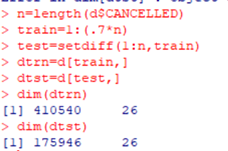
This post, I will be testing my logistic regression model that I built in my previous post. I will test for accuracy and stability, similar to what I did to my linear regression model. Just like in my linear regression post, the data will be split into a testing and training set, but I will use the latest set of data because my data is an observation over time. I would use random sampling if my data was people or items. Through splitting my data into two sets, I am able to compare the predictions which helps conclude if my model is stable and accurate. Below is how I divided the data.
I have created two new sets from that code. The two sets are training of 410,540 observations and testing of 175,946 observations.
Next I will predict cancelled flights in my training set using my logistic regression model:
All of my predictors are significant, which is great because I can move forward with my model using my complete model. My model equation for my test set is: log(p/(1-p))=-3.22-0.09*dayofweek-0.18*month where p is the probability of a cancelled flight.
From this equation, I am able to make predictions with the code below.
The next code I will use is labeling yes or no predictions with a zero or one. This will better help me compare.
I can now use a confusion matrices to really compare what was predicted and what actually happened. The code and output of these matrices are shown below.
This model is both stable and accurate. First let’s talk about stability. When comparing the training and the test set, the numbers are off by a few decimals. A few decimal places is very good. My model being stable is great. Now let’s check for accuracy. I was 98% right most of the time. This means, when predicting a flight was not cancelled, I was right 98% of the time that it was not cancelled. When predicting a flight wasn’t cancelled but actually was, I was wrong 2% of the time. Being wrong 2% of the time is a very small number, and we are predicting flights. I would say this is not a huge problem because it is not a life or death situation. Additionally, I was right 98% of the time which is almost close to perfect accuracy. From this information, I would say my model is accurate.
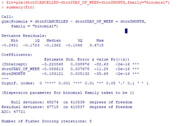
In my previous post I created a model to predict a binary variable. Similarly to the assumptions I tested for linear regression, I will now do the same but with logistic regression. The model and code I created is shown below.
The model equation is:
log(p/(1-p))=-3.14-0.01*dayofweek-0.17*month with p being the probability of cancellation.
The first check of assumptions is to have a good linear model. This means, all the variables I have included in my equation are significant. They are all relevant to my equation so this is checked off.
I must now make sure there is no perfect multicollinearity between the x and y variables. A perfect mulitollinearity is indicated by 1. I must test both x variables because they are both significant. I used the code below to test this assumption.
There is no perfect multicollinearity in this model which is awesome. Additionally, both -.003 and -0.06 are between the range of -0.25 and 0.25 which is good! This means the two variables are not very alike and will allow us to use them as predictors without a problem. This assumption test is passed.
Assumption 3 is independent errors. Independent errors for logistic regression is only intuition. My intuition tells me each flight and airline are all independent of each other, meaning it passes the test of independent errors
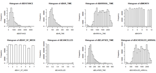
Next is assumption 4 which is complete information. I have used the code below to output histograms of each variable.
The histograms help me visually see how the data is distributed. It also allows me to see if I have enough data. From the graphs, I think our data is pretty fairly distributed. The graphs show a variation of frequencies which is good because it mean there is many observations for each variable. There is a great range of data. I also believe there is a good amount of data. The model passes this assumption of having complete information.
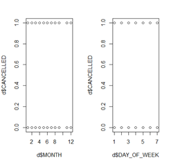
The next assumption is complete separation. I will test for that with a scatter plot. Below is the code and output received.
This plot shows me no vertical line can be drawn between month and cancelled along with cancelled and day of week to separate them, thus this model does not suffer from complete separation. My model passes this assumption.
The last assumption is large sample size. My data has 586,486 observations which is a huge sample size. I would say my model passes this assumption with the large size of it’s sample being over 500 thousand.
My model has passed most of these tests which is great!
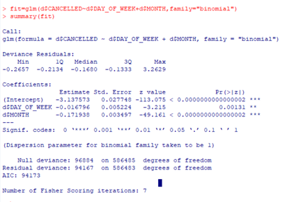
I have now learned how to create model equations with binary variables. I used the binary variable of cancelled to be my Y, or what I am predicting. My X variables, or the predictors, are day of the week and month. The code I used to create my model is shown below along with the output.
All of my predictors are significant, the stars indicate this, so I can move forward with my model equation using the intercept and both predictors.
My model equation would be:
log(p/(1-p))=-3.14-0.016*dayofweek-0.17*month where p is the probability of the flight getting cancelled.
When the day of the week or month does not matter, there is a low chance the flight is getting cancelled. I know this because a log odds ratio around -3 is a low probability, similarly a negative slope means you would “move down the line” meaning a lower probability.
Lastly, the probability of a flight being cancelled is less likely to be affected by the day of the week. I know this because this number is a negative number meaning the day of the week decreases the chance of the flight being cancelled. Additionally, the month is also less likely to affect cancellation of flights. The negative in front of the number indicates the month will decrease the chances of cancellation.
Hello everyone! Thanks for following along this far! I have developed a lot more analytical skills I will now practice and show you all what I have learned.
In this post, I will be using a test set and training set to analyze how well my model can predict. I am doing this because a training set will be used to help build the model and a test set to use on the model I have already created that will help test it.
My data is organized as observations over time, so I will use the latest data set as my tester. The code below is how I divided the data:
The divided data came out to be:
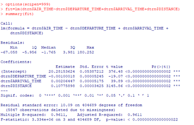
Next I will use the training set to build my model, which then created this output:
The model equations is:
air time= 20.28-0.001*departuretime+0.002*arrivaltime+0.10*distance
The model is different than previous posts because only 70% of the total data is being used for this prediction, and the other 30% will be used for the testing set.
Next I will create predictions and errors for the test set from my model equation just created with the training set.
I will now create a histogram of these errors to get a better understanding of these errors visually. Through doing this, I will be able to conclude if my errors are stable and accurate.
Shown below if the histogram output I got from my code.
I am now able to see if my model is accurate and stable. First, let’s talk about accuracy. My model is about 7 minutes off when talking about airtime. 7 minutes could be the difference between a 3 hour flight, and a 4 hour flight. In that perspective, it seems as though it is a big difference. Additionally, 7 minutes could be the difference of a pilot or flight attendants pay. Although it does not seem like a lot, getting paid for a full hour and not getting paid for a full hour, could be a decent difference in pay. Another issue with these is a passenger needing to get on a connecting flight. Sometimes, connecting flights can be within a half hour of when your plane lands, possibly even less time than that. In that sense, time is everything. A passenger who gets off the plane 7 minutes later than anticipated, could possibly miss his flight. With all this being said, I believe this model to be inaccurate
Now we’ll talk about stability. The two histograms differ very much between each other. The first histogram is centered around zero which is great. However, the second histogram is spread between 0 and 200. This means it is unstable.
My model is both unstable and inaccurate, which is NOT GOOD!! However, I will learn new tools to help combat this.See you next time!
Welcome back everyone! This post I will be testing the 5 assumptions of linear regression using my model equation with the variables distance, arrival time and departure time. Here is the model equation: Air Time= 19.86 + 0.1108*Distance – 0.0010*DepartureTime + 0.0021*ArrivalTime. The R-Squared of the model is 0.953.
Let’s get started with the assumptions! We will not test assumption 1 and will go right to assumption 2.
Assumption 2: Assumption 2 has to do with multicollinearity. The model must not have a perfect multicollinearity, which is represented by a 1 or -1. This model does not have any of that, thus there is no perfect multicollinearity in this model. The first assumption is checked off. The data, of correlation between the variables, is shown below.
Assumption 3: Assumption 3 is independent errors. There are 3 tests within this. The first test is intuition. My intuition tells me we are studying flights from different airlines and different types of planes, thus they are independent of one another. The next test is plotting the residuals, identifying that there is no pattern within that. The code I use to plot this is shown below along with the output.
This graph seems to be a bit concerning. The errors do not seem to be randomly distributed, as there is a lot of overlap between the errors, causing this solid black coloring. The errors are distributed between 0 and 50 however, there seems to be random distribution at 0 from 100,000 to 300,000, but then from 300,000 to 500,000 the distribution switches to 50. This makes me question the significance and the independence of the variables. The model does not pass this test.
Next, I will test the auto correlation with an ACF test. The code for this test is:
The output I got is:
This output is very concerning. Each lag passes the blue line threshold meaning they they are significant. This raises my concern, because it is not one or two lags that pass through the blue line, it is all of them. This means, there is correlation between each error.
After testing my model using graphs and intuition, my model does not pass assumption 3.
Now onto assumption 4.
Assumption 4 tests the heteroskedasticity. Similar to the last assumption, there are a few tests that go into this assumption. The first one is to plot x and y and the second is to test for random distribution. The code to plot this is:
The graphs do not pass the heteroskedasticity test. I know this because as I move from right to left on the graph, there is a wide difference in variance across each variable. For example, distance vs air time shows a pretty constant variance, but then there is suddenly nothing, showing a change in the variance. In order to pass heteroskedasticity, there needs to be an equal variance across variables. Secondly, the model fit$resid v fit$fitted will plot errors versus predicted values. Here, we are looking for a graph in a circular shape, with random distribution. My graph shown on the bottom right, is not that circular shape and is rather in straight, horizontal lines. There is no randomness to it.
Unfortunately these tests proved that my model does not pass assumption 4 of no heteroskedasticity. Instead, my model is heteroskedastic, and has unequal variances.
Finally, the 5th and final assumption, normally distributed errors. There are 4 possible tests within this assumption, however my model only needs to pass one of them to meet the assumption. I am going to plot all four just in case. The code I will use is below:
I can immediately tell the model does not pass these tests or assumption 5. First, the histogram of air time is skewed mostly to the left, not showing a normal distribution that would be in the shape of a bell. The distribution is mostly to one side. Additionally, the Q-Q plot also helps me see this violation. A perfectly normal distribution would show a straight line. I plotted a line to show if my points were straight, which clearly shows they are not. If the Q-Q graph was a straight line, the points would be hugging that line. My model violates yest another assumption.
Although my model violates 3 out of 4 assumptions, I can still move on with my model. These violations tell me there are correlations within variables along with variables not being significant. They tell me that the significance of variables is questioned. I will still move on with my model even though there are violations, because I need to practice my skills and I am not in a real life situation. There are ways to fix these violations, yet that is a skill that the scope of my course does not cover. If this were a real life situation I would be able to fix those violations.
Recently, I have been using a model equation with 3 variables as predictors. The three variables are distance, and arrival and departure time. My model equation from this is: Air Time= 19.86 + 0.1108*Distance – 0.0010*DepartureTime + 0.0021*ArrivalTime.
I will now test the correlation between these three variables. In order to do this, I will use the code below:
This code gave me these results:
This code helps me see the correlation between the 3 variables in an organized fashion. I will not interpret what this chart means and the correlations between all the variables.
The correlation between distance and arrival time is 0.04 which does not raise any question of correlation as the number is exactly what I;m looking for.
Next, the correlation between distance and departure time is 0.002, which is again a small enough number to not have concern of them being correlated.
Lastly, the correlation between arrival time and departure time is 0.76 which raises some question. The number is a little big for multicollinearity. This means the two variables have a correlation, which will make it hard to interpret their slopes.
My model partially suffers from mutlicollinearity with 4 out of the 6 variable pairings not being affected, however 2 variables, arrival and departure time, are affected by it.